Hands-on, part 1

In this hands-on assignment, each group shall create a mesh with the object to simulate. Some groups are assigned a sphere, while others are assigned a cylinder (announced on your Slack channels). We consider a plasma similar to the F-layer of the ionosphere, with the following parameters.

Electron and ion density: 1e11 /m^3
Electron and ion temperature: 1000 K (=0.08617 eV)

The object has the following dimensions:

Sphere: Radius of 0.5 electron Debye length
Cylinder: Radius of 0.2 electron Debye lengths, and a length of 10 electron Debye lengths

You may find the files in the Geometry folder helpful to start with. Let the outer boundary be of the same shape as the object, but extending 10 electron Debye lengths beyond the object in every direction. The resolution on the outer boundary can be taken to be 1.5 electron Debye lengths, whereas on the inner boundary it should be a fifth of the radius. Let the lower and upper half of the object be two distinct physical groups, such that different voltages can be assigned to them in PTetra.

The mesh will be used for simulations in the next assignment. Although each group only needs one mesh (to begin with), we encourage all participants to try creating this mesh, asking their group for help before asking the organizers.

Step by step guide to generate mesh for spherical probe

First open the sphere_0.5R.geo file using any of your text editor. We are going to use Vim as text editor throughout this guide. Feel free to use your preferred editors like Atom, gedit, nano if you feel comfortable. Make sure you are inside the Geometry directory before you do so. You can check it by typing the command pwd.

vim sphere_0.5R.geo

It should look like,

// STEP 1: SET VARIABLES

debye = 0.00690; // Electron debye length for n=1e11 and T=1000
r = 0.5*debye;   // Inner radius
R = TDB;         // Outer radius
Res = TDB;       // Resolution on outer boundary
res = TDB;       // Resolution on inner boundary

// STEP 2: PLACE POINTS (0D ENTITIES)

// Center
Point(1) = {0, 0, 0, Res};

// Outer boundary
Point(2) = {R, 0, 0, Res};
Point(3) = {0, R, 0, Res};
Point(4) = {0, 0, R, Res};
Point(5) = {-R, 0, 0, Res};
Point(6) = {0, -R, 0, Res};
Point(7) = {0, 0, -R, Res};

// Inner boundary
Point(8) = {r, 0, 0, res};
Point(9) = {0, r, 0, res};
Point(10) = {0, 0, r, res};
Point(11) = {-r, 0, 0, res};
Point(12) = {0, -r, 0, res};
Point(13) = {0, 0, -r, res};

Change the radius and other parameters (as well as TDB) to your problem specific values. For the demonstration we are plannig to design a spherical probe with radius 0.5xdebye length. To be able to edit the file using Vim, press I or the Insert key on your keyboard.

// STEP 1: SET VARIABLES

debye = 0.00690; // Electron debye length for n=1e11 and T=1000
r = 0.3*debye;   // Inner radius
R = r+10*debye;         // Outer radius
Res = 1.5*debye;       // Resolution on outer boundary
res = r/5;       // Resolution on inner boundary

// STEP 2: PLACE POINTS (0D ENTITIES)

// Center
Point(1) = {0, 0, 0, Res};

// Outer boundary
Point(2) = {R, 0, 0, Res};
Point(3) = {0, R, 0, Res};
Point(4) = {0, 0, R, Res};
Point(5) = {-R, 0, 0, Res};
Point(6) = {0, -R, 0, Res};
Point(7) = {0, 0, -R, Res};

// Inner boundary
Point(8) = {r, 0, 0, res};
Point(9) = {0, r, 0, res};
Point(10) = {0, 0, r, res};
Point(11) = {-r, 0, 0, res};
Point(12) = {0, -r, 0, res};
Point(13) = {0, 0, -r, res};

Save the file in Vim using the following sequence Esc,:,w,q,!,Enter.

Next, open this .geo file by using the following command in your terminal,

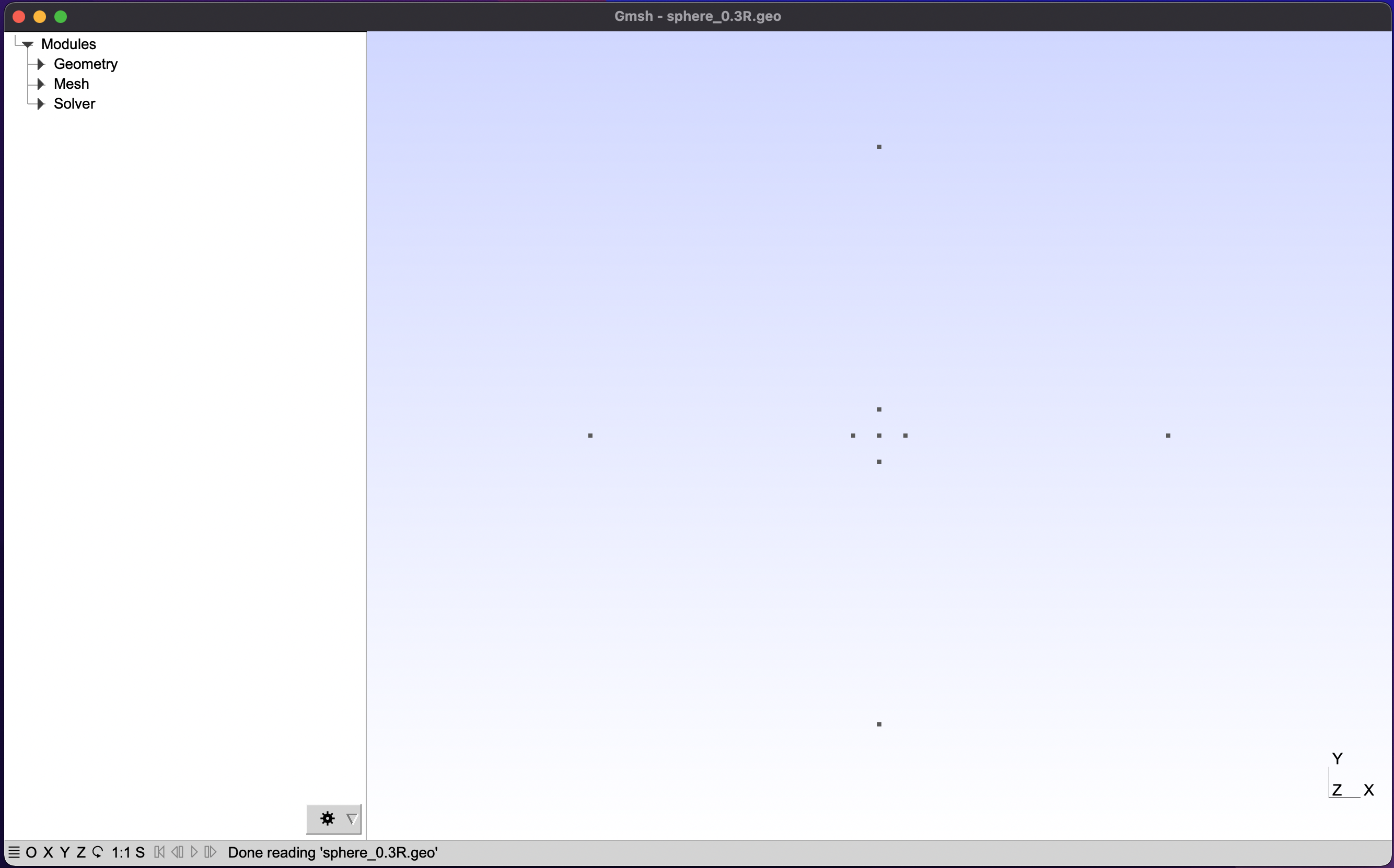
gmsh sphere_0.5R.geo

It should open up a window like the following,

gmsh1 Click on the left menu in the following order: Geometry->Elementary entities->Add. At the end of this your left window should look like the following,

gmsh2

Note: From now onwards in this section our mostly used tools will be Circle arc, Surface filling, and Volume.

First rotate your geometry with a view where you can see the different planes.

gmsh3

Geometry

Elemetary entities

Circle arc

Next, choose Circle arc from the left menu and select the first point on your outer sphere to make a arc. Then the centre of the sphere followed by the end point of the arc. Note:

Circle(id) = {start, center, end};
id: unique id assigned to each element with a specific type 
start, end:start and end points of an arc
center: center of the arc/circle

gmsh4

Now repeat the same for all the arcs on the outer sphere. By the end, it should look like the following,

gmsh5

Now, we need to do the same for the inner sphere. The first step should be similar. Note: make sure to zoom in to have a clearer view.

gmsh6

Now, try to connect all the points forming arcs on the inner sphere (probe). The final product should look like,

gmsh7

Now, press q to come out of the Circle arc action.

Next,

Surface filling

Choose Surface filling from the left menu and select the first arc on your outer sphere. Then, continue to select the next two arc forming a curve surface segment of a sphere. Finally, end the selection by pressing the key E on your keyboard. After pressing E, you should be able to see a faint dotted curve forming the surface you just created.

gmsh8 gmsh9

Now, repeat the process for all the curved surfaces on the outer sphere. The final product should look like,

gmsh10

Next, repeat the same for the inner sphere. Remember to zoom in before you select the arcs to form the surface.

gmsh11 gmsh12

Now repeat the same process for all the curved surfaces of the inner sphere. The final product should look like,

gmsh13

Next,

Volume

Choose Volume from the left menu and select the dotted curved surface line on the outer sphere first followed by the dotted curved surface lines on the inner sphere. Press E to end the selection. In the end the you should be able to see a yellow round ball at the centre.

gmsh14 gmsh15

Press Q to abort and exit the action.

Next,

Physical groups

Surface

Expand the Physical groups tree on the left menu to see available groups. Choose Surface and select all the curved sufaces on the outer sphere by clicking on the dotted lines. Press E to end the selection. gmsh16

Now, repeat the same for the inner sphere. Complete the selection by pressing E in the end.

gmsh17

Press Q to abort and exit the action.

Note: If you need segmented biased probe. Select the top half of the inner sphere and bottom half of the sphere separately.

Next,

Volume

Choose Volume and select the yellow sphere at the centre. After selection the Yellow sphere becomes Red. Press E to end the selection. Finally, press Q to abort and exit the action.

gmsh18

So, we have now finished our Geometry. Next,

Mesh

Go to the Tools menu on the top left corner and click on Options. Then click on Mesh on the left and open Advanced tab. Check the box named Optimize quality of tetrahedra with Netgen. Remember to click on Save Options as Defaults before closing Gmsh.

netgen_gmsh_1 netgen_gmsh_2

Now, to generate 2D mesh, go to the left panel and click on Mesh and click on 2D.It will generate 2D Mesh on the surfaces that we declared.

gmsh19

Now, click on 3D to generate 3D volume mesh.

gmsh20

To understand the quality of the mesh, Go to the Tools menu on the top left corner and click on Statistics. mesh_statistics stats_details

Thin cells lead to less accurate solutions and slower convergence. The value of quality factor, gamma indicates how regular the cells are. Gamma(γ) = 1 represents a perfect equilateral, and gamma = 0 represents a degenerate cell. The higher the average, better the mesh quality. For simple geometries, the lowest gamma value could be 0.3 or above but for complicated geometries it also can be less than 0.05.

You can also plot the statistics data.

mesh_q_plot

Now, we are all done. Let’s export the mesh.

Go to the File menu on the top left corner and click on export. The default save as option should be Guess from Extension(*.*) Use .msh extension and choose Version 2 ASCII when prompts to save. gmsh_menu

For our case we saved the Mesh file as sphere_0.5R.msh.

Now, edit msh2topo.dat using Vim or any of your text editors.

vim msh2topo.dat

It should look like,

inputFormat: 'gmsh1', 'gmsh2', 'abaqus1', abaqus2' or 'spis'
outputformat: 'Vu' or 'topo'
&readoptions
  inputFormat='gmsh2'
  outputFormat='topo'
/

$begin
nfields=0
sphere.msh
$end

Now replace the mesh file name to your own sphere.msh->sphere_0.5R.msh.

inputFormat: 'gmsh1', 'gmsh2', 'abaqus1', abaqus2' or 'spis'
outputformat: 'Vu' or 'topo'
&readoptions
  inputFormat='gmsh2'
  outputFormat='topo'
/

$begin
nfields=0
sphere_0.5R.msh
$end

Then, save the file. Now, run msh2topo

./msh2topo

The output should look something like this,

call readMeshGmsh2
 sphere_0.3R.msh
 nv=         892
 netot=        3789
 ne1=           0  ne2=         232  ne4=        3557
 i1=           0  i2=         232  i4=        3557
 call buildNeighbours
 i1=           1  j1=           4
 i1=           3  j1=           4
 i1=           7  j1=           4
 ...           .  ...           .
 i1=        3554  j1=           1
 Test the mesh for duplicate neighbours
 Test the mesh for consistent adjacency
 call readFields
 call outputTopo

Once it is over, you should be able see a file name msh2topo.out. Rename the file to a convenent one with .topo format.

mv msh2topo.out sphere_0.5R.topo

That’s all!!!